Topology and Edge States
We recently published a paper in Physical Review Letters on a new topological invariant for edge states in simple, one-dimensional models. The arXiv version is also available here.
General summary
Topological physics studies properties that stay the same even when a system is smoothly deformed, with different phases labeled by integers (called topological invariants). This area has led to three Nobel Prizes (1985, 1998, 2016). One of the simplest examples appears in 1D lattice models, where topological “edge states” (states localized at the ends of the lattice) can form. Traditionally, such topological phases for edge states were thought to require certain symmetries to exist in 1D. We prove that a new topological invariant can be used for simple asymmetric 1D models that predict edge states. It reduces to the well-known symmetry-protected case when symmetries are present.
Topological invariants
For the rest of this blog post, it helps if you’re familiar with the Su-Schrieffer-Heeger (SSH) model. There already exist other nice tutorials on this such as here, here. and here.
Fig 1 shows the topological invariant for edge states for three models: the SSH model (Fig 1a), an asymmetric Hermitian model (Fig 1b), and an asymmetric non-Hermitian model (Fig 1c).
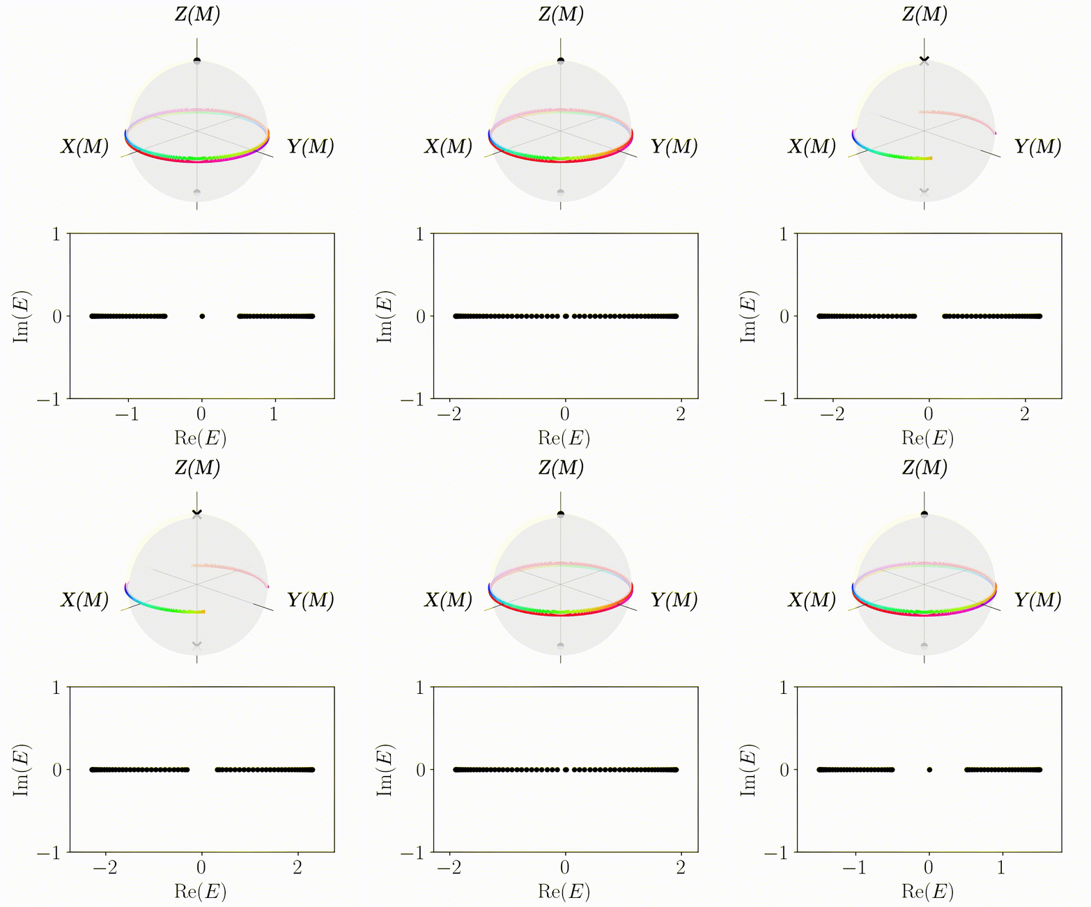
Fig 1a (top) Topological invariant and (bottom) open boundary condition eigenvalues for Hermitian SSH model.
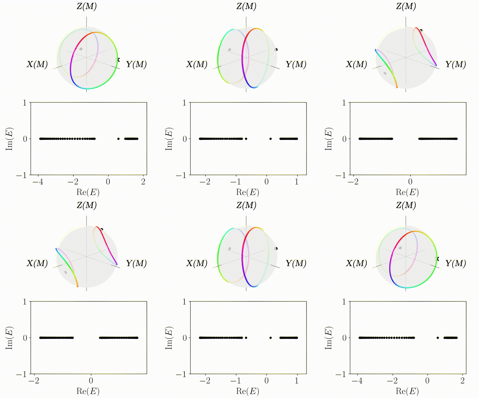
Fig 1b (top) Topological invariant and (bottom) open boundary condition eigenvalues for a Hermitian asymmetric model.
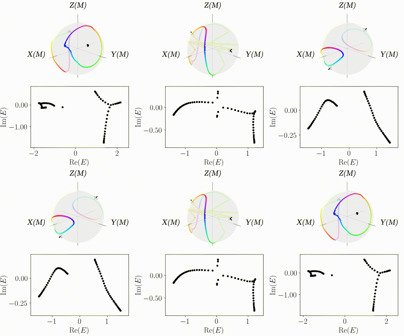
Fig 1c (top) Topological invariant and (bottom) open boundary condition eigenvalues for a non-Hermitian asymmetric model.
The SSH case is the well-known textbook case. The second and third columns are the new invariants from our paper for simple asymmetric 1D models.
SSH model
It is easier to explain our asymmetric model edge state invariant by building on the SSH model intuition, so we briefly review the SSH model which is a simple tight-binding chain with alternating bonds (Fig 2).
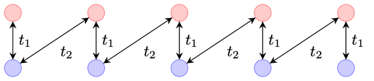
Fig 2 SSH model with alternating bonds.
In Fig 3, we show the open boundary condition eigenvalues of the finite chain with \(N=32\) unit cells as well as the band structure of the model.
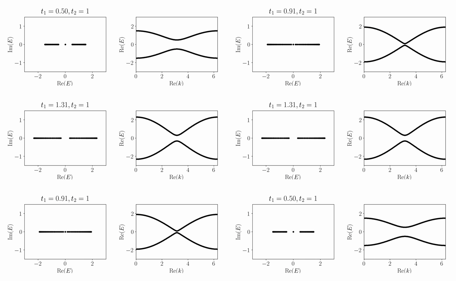
Fig 3 (left) Open boundary condition eigenvalues for finite chain with N=32 unit cells and (right) corresponding band structure.
Although the band structure plot on the right is common in Hermitian studies, we will look at some non-Hermitian models, and so the format of the left plot is convenient for us. The open boundary eigenvalues also has all the band structure information when \(N\) is large enough anyway, see Fig 4.
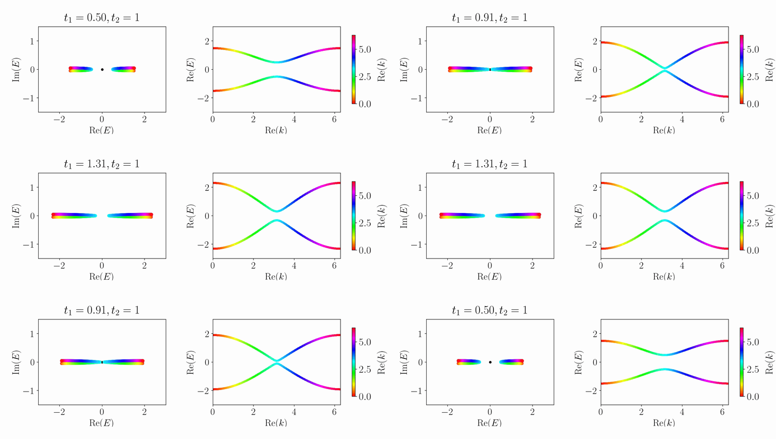
Fig 4 Same as Fig 3 but colored by Re(k) which is the direction of the integration contour for topological invariant.
The topological invariant (called the Berry-Zak phase) is plotted on the right in Fig 5 on the Bloch sphere. When the band winds around the north and south pole axis on the edge state, there are edge states. When it does not wind, there are no edge states.
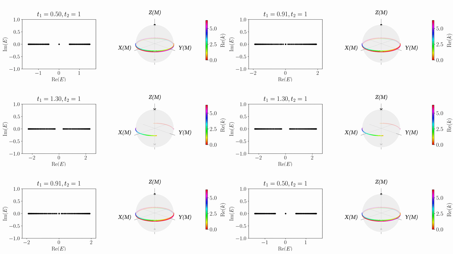
Fig 5 (right) SSH model topological invariant on the M-Riemann sphere, which is the same as the Berry-Zak phase on the Bloch sphere.
Bloch sphere
We define the Bloch sphere in a slightly different way, with \(X(Y), Y(M), Z(M)\) coordinates in Fig 6. It is equivalent to common Bloch sphere definitions for Hermitian models - see left and middle panel in Fig 6. All three representations use the Bloch Hamiltonian, which applies to systems with translational symmetry:
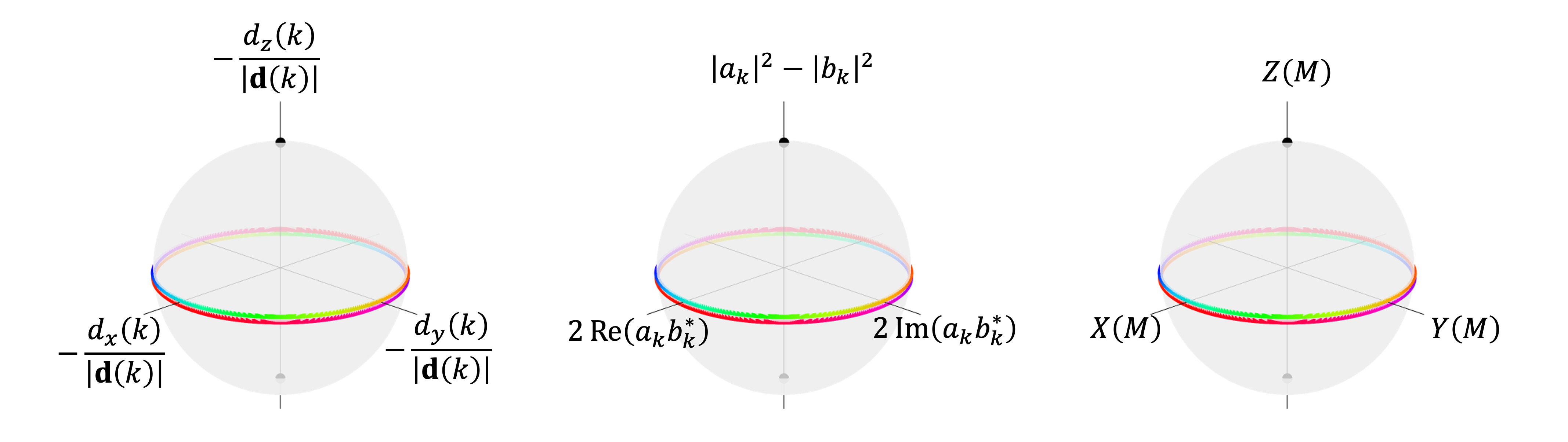
Fig 6 Bloch sphere representations.
The left plot uses the Hamiltonian \(d\)-vector \(H(k)=\sum_{i=0, x, y, z} d_i(k) \sigma_i\) where \(\sigma_i\) is the Pauli matrix (example here). The middle plot uses Bloch eigenvector components (example here). In the right, we define the eigenvector ratio \(M(k)= a_k/b_k \in \mathbb{C}\). We can compactify \(M\) onto a sphere, and that is the \(X(Y), Y(M), Z(M)\) coordinates of the \(M\)-Riemann sphere. This \(M\)-Riemann sphere form is nice because all the eigenvector information is in a single complex number \(M\).
Asymmetric Hermitian model
We will consider 1D tight-binding models with nearest neighbour interactions between unit cells (which includes some but not all third nearest sublattice neighbour hoppings). This model can be demonstrated in cold atoms in a lattice, electrons in a chain, light propagation in photonic waveguide arrays and more. It also includes the SSH model, Creutz model, Rice-Mele model and more.
We are interested in the case where we choose random Hermitian couplings and on-site energies. Consider the model \(H_{h,rand}\):
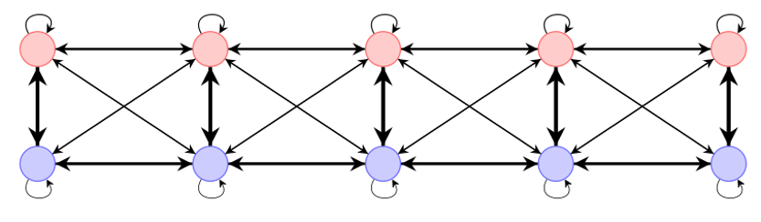
Fig 7 Hermitian nearest-neighbour model with random couplings and on-site energies.
In Fig 7, I tried to show the couplings of \(H_{h,rand}\) where the thickness/ arrow head size is roughly the weight of the coupling or on-site energy. Note that we still have translational symmetry (periodicity) but we have broken chiral, time-reversal and particle hole symmetry. This is class A in Kitaev’s classificaiton table which is no symmetry in that table, so we call it an asymmetric Hermitian model.
The topological invariant for a family of Hermitian models is shown in Fig 8. We are using \(H_{\mathrm{h}}=(1-\alpha) H_{\mathrm{h}, \text { rand }}+\alpha H_{\mathrm{ssh}}\) where \(t_2=1\).
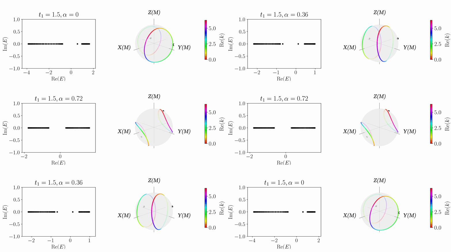
Fig 8 Asymmetric Hermitian model open boundary modes (left plot) and topological invariant on the M-Riemann sphere (right plot).
Unlike the chiral symmetry case, asymmetric model edge states do not have to be at \(E=0\). In the above, we have 0, 1 or 2 edge states. When the two dots are in the loops on the sphere on the right plot, there are two edge states. When one is in the loop, there is one edge state. When neither are in the loop there are crosses and there are no edge states. This is our topological invariant we introduce in the paper.
We will unpack the right side of Fig 8 - namely what are those two points that the loops are winding around? They sit on the north and south pole axis for the SSH model but can move around the sphere for the asymmetric model.
General wave-function
To know where they come from, it helps to know where edge states come from. The general solution for a nearest-neighbour tight binding model wave-function with arbitrary boundary conditions is given by the generalized Bloch ansatz:
where \(\left|z_1\right| \leq\left|z_2\right| \leq\left|z_3\right| \leq\left|z_4\right|\) and \(z=e^{i k}, k \in \mathbb{C}\). Using \(z\) is nice because it makes things into polynomials. A simpler example of the generalized Bloch theorem are the edge states of a SSH open boundary model. The edge states are a linear combination of a left and right edge (which is a \(z\) term with \(\left|z\right|<1\) and \(\left|z\right|>1\) respectively). For this nearest-neighbour model, the equations of motion are a fourth order linear recurrence equation, so we have four terms. The solution above is just a \(z\)-transform, which is like a Fourier transform but with complex \(k\) allowed. We also label the eigenvector term \(M_i\) according to the \(z_i\) it belonged to.
Bulk eigenvector degeneracy
We introduce a new concept which we call a bulk eigenvector degeneracy. It is when two of the eigenvector terms in the general wave-function above point in the same direction. An example is:
where \(\color{green}M_1=M_2\). This condition is very relevant because it turns out edge states are bulk eigenvector degeneracy points.
To briefly see why, we apply open boundary conditions \(\psi_{n a}, \psi_{n b}=0\) for \(n=0, n=N\) which gives us four equations which we can write as a matrix equation:
Call the above matrix \(B\). For valid solutions, we need \(\operatorname{det}(B)=0\). It is easy for \(\operatorname{det}(B)\) to blow up since we have \(z\) magnitudes that can be larger than 1 and \(N\) can be arbitrarily large. The leading terms of \(\operatorname{det}(B)\) are:
In order for this to not blow up when \(N \rightarrow \infty\), there are two kinds of solutions. The first is that \(M_1 =M_2\) or \(M_3 =M_4\) which are the edge state solutions. The other way is for \(\left\vert z_2\right\vert = \left\vert z_3\right\vert\) which are the bulk states (called the generalized Brillouin zone) which are the continuum open boundary condition bands.
From the Bloch equations (which are just some polynomial equations) and some algebra, we can use the condition for bulk degeneracy points and find that there are are always two \(M_{\text{deg}} \equiv M_{i}=M_{j}\) solutions for a nearest-neighbour model - so there are always two bulk eigenvector degeneracy points, but they may or may not be edge states.
So, to summarize:
where \(\color{green}M_1=M_2\) and
where \(\color{green}M_3=M_4\) are edge states. But
where \(\color{red}M_1=M_3\) is a bulk eigenvector degeneracy but is not an edge state.
We can solve for where these two bulk eigenvector degeneracies occur and we plot this in green if it is an edge state and red if it is not in Fig 9. We can also find the eigenvector ratio \(M\) where these degeneracies occur and plot them on the \(M\)-Riemann sphere. That’s what those two dots or crosses are in the right plot - the topological invariant is about the bulk eigenvector degeneracy points.
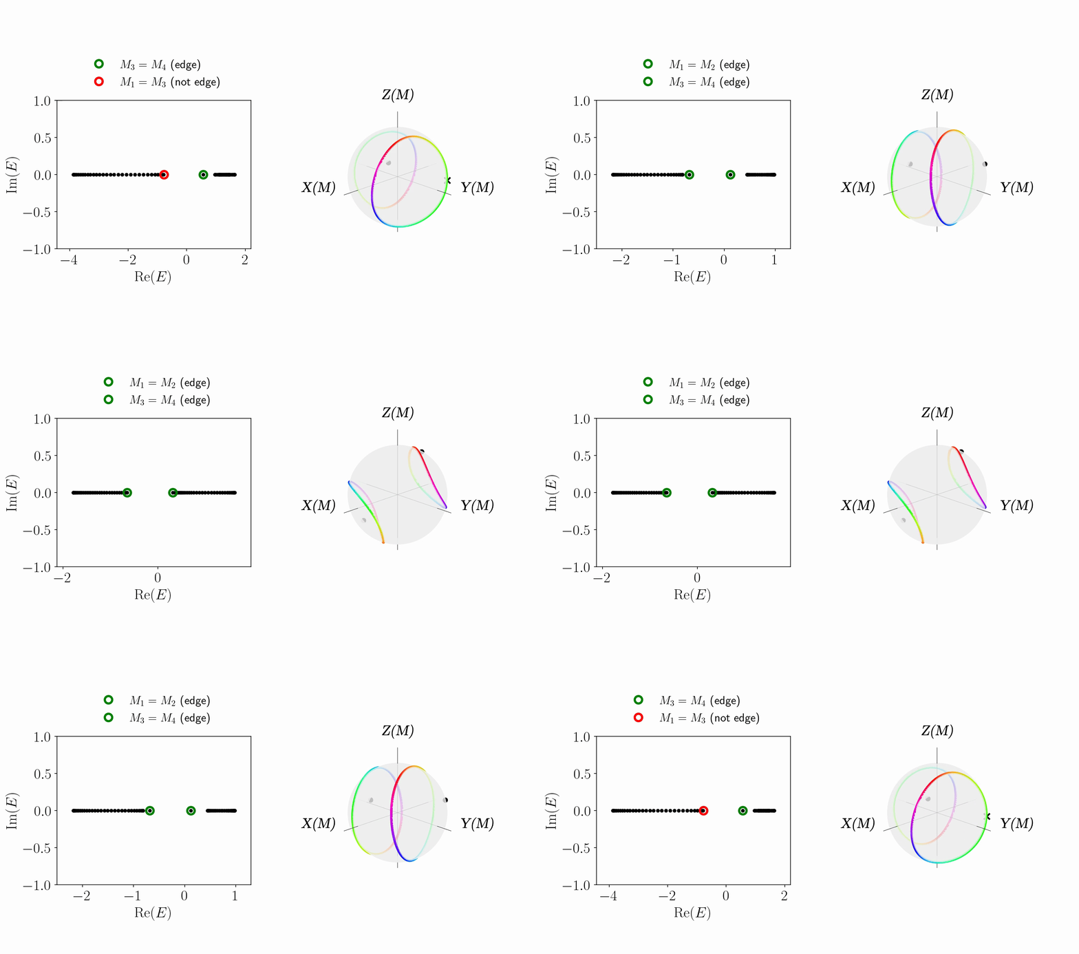
Fig 9 Same as Fig 8 but with red or green circle to showing bulk eigenvector degeneracy points.
We can see that the transitions match very well. In the right plot, the topological invariant is a fancy index tracker that tells you whether the bulk eigenvector degeneracy points have the correct indices for edge states. These indices change into and away from the edge state condition when they cross the loops on the sphere. This is because the loops are the continuum open boundary condition bands. They are where the \(z_2\) and \(z_3\) sheets meet (and therefore also where the \(M_2\) and \(M_3\) regions meet), so a bulk degeneracy point changing from eg \(M_1=M_3\) into \(M_1=M_2\) or vice versa must cross that line.
It is useful to write this as a formula. The topological invariant for our asymmetric nearest-neighbour Hermitian model is:
The main thing is that the invariant is now about the bulk degeneracy point. In Fig 10, we also include the \(M\)-plane in the middle plot which is just the uncompactified version of the right plot, and where we typically calculate the invariant. The mod 2 makes it just a parity check, we do not need to care about the direction of winding.
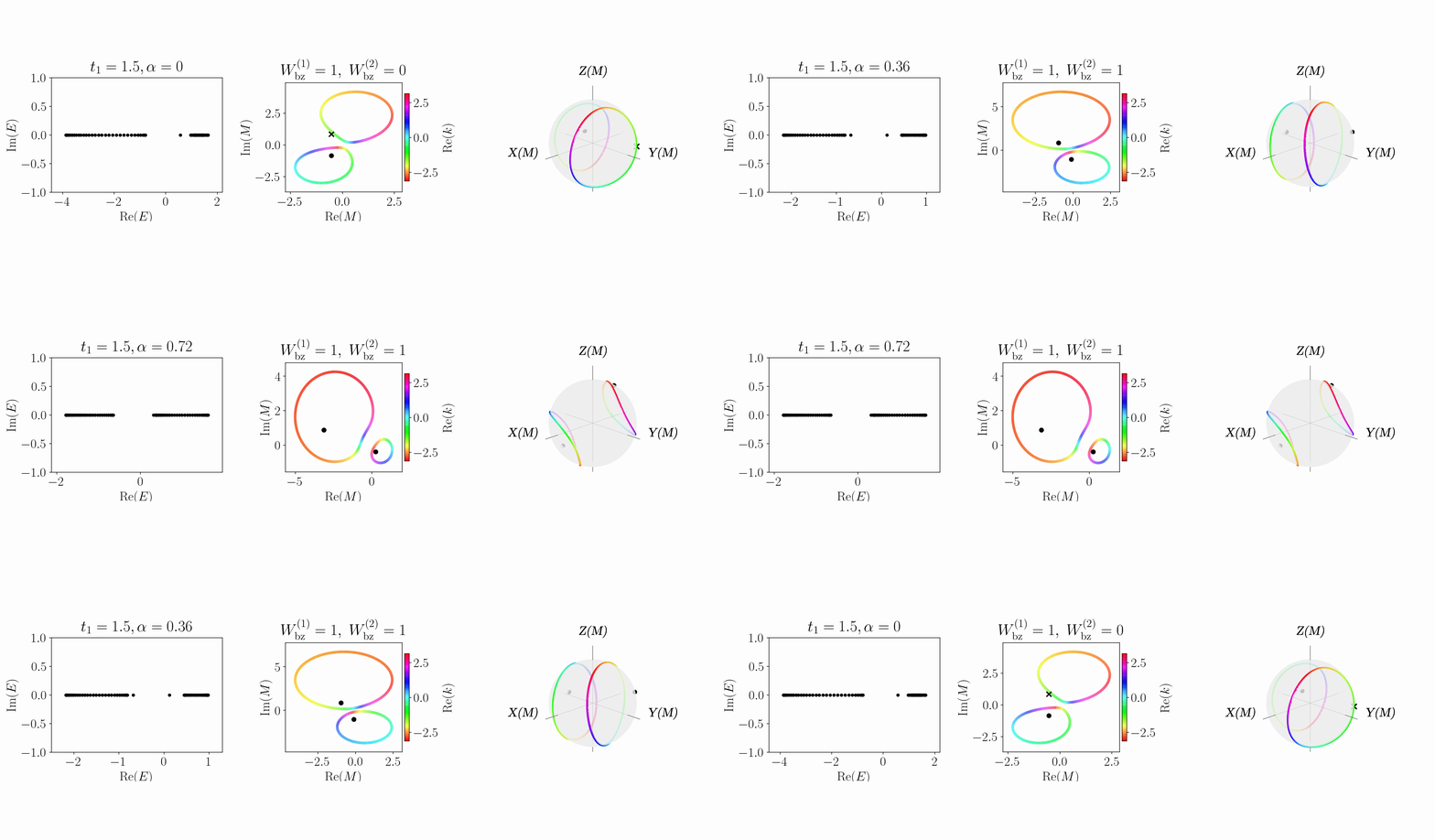
Fig 10 Same as Fig 8 but also with M-plane version in the middle.
It is useful to check it reduces to the correct invariant when chiral symmetry is applied. When we have a case with chiral symmetry (and the Bloch Hamiltonian is in off-diagonal form), the asymmetric model edge state invariant reduces to the familiar Berry-Zak phase, as seen in Fig 11.
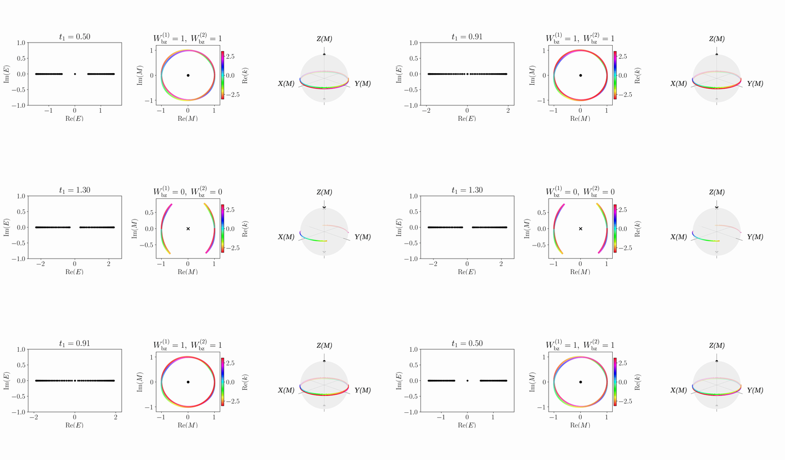
Fig 11 Same as Fig 5 but with M-plane plot in the middle.
The \(M_{deg}\) points go to 0 and \(\infty\), and the winding number becomes:
which is equivalent to the Berry-Zak phase. The middle plot in Fig 11 is the same as the SSH \(d_x, d_y\) winding number that some people use in the literature.
Asymmetric non-Hermitian model
We also consider a non-Hermitian model, \(H_{nh,rand}\):
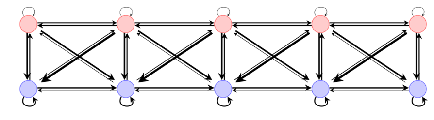
Fig 12 Non-Hermitian nearest-neighbour model with random couplings and on-site energies.
All the same intuition applies. The edge state condition and the bulk eigenvector degeneracy formulas are the same. Edge state transitions still occur when the bulk degeneracy point moves in and out of the loops on the \(M\)-Riemann sphere (see Fig 13).
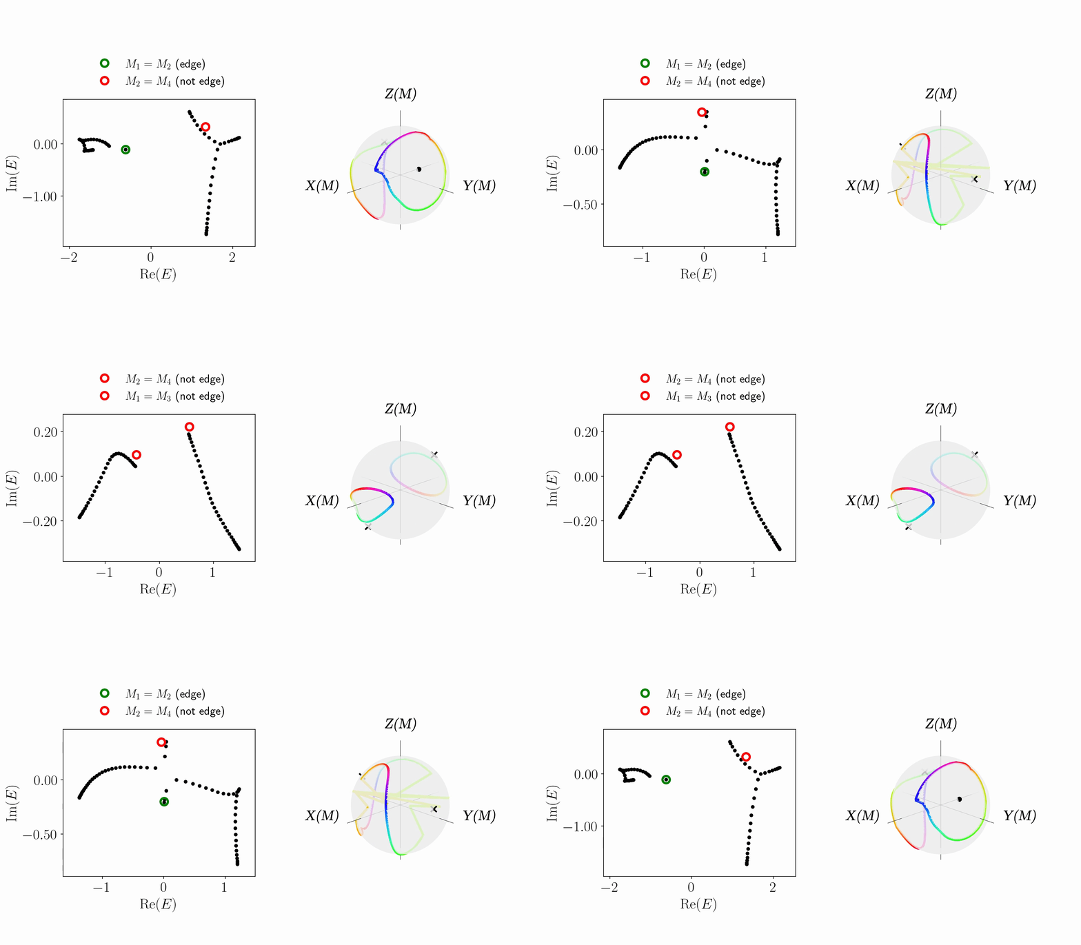
Fig 13 Asymmetric non-Hermitian model bulk degeneracy points in red and green, open boundary modes in black (left plot) and topological invariant on the M-Riemann sphere (right plot).
Unfortunately, some weirder things can happen in non-Hermitian models. One example is that since the bands have complex energies, they may braid. They also may not even be a braid. The bands can intersect and merge on the \(M\)-Riemann sphere. To keep track of the orientations of the loop and the regions they define, we also have to include the branch points on the \(M\)-plane which we plot as red dots in Fig 14.
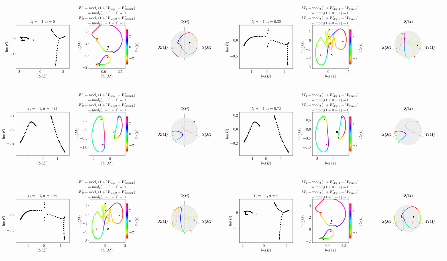
Fig 14 Same as Fig 13 but also with M-plane version in the middle and M-plane branch points in red.
The topological invariant for non-Hermitiam asymmetric nearest-neighbour models is:
If you are only interested in Hermitian systems, you can ignore this one. However, it is worth noting that this is the more general formula and that the Hermitian one is a special case of this one. I will try to give an essence of the proof of this above formula and why the \(M_{branch}\) points matter. This formula, the proof of it and the original animation in the next section is credited to co-first author Heming Wang.
Proof of the edge state invariant
Although we will try to give an essence of the proof of the non-Hermitian asymmetric edge state invariant, we will use a Hermitian example to keep terminology simple.
While we normally plot band structures in real energies \(E\) and real momentum \(k\), the full picture, for both Hermitian and non-Hermitian models is that the band structure is complex where \(E, z \in \mathbb{C}\). For this nearest-neighbour model, the orders of \(E\) and \(z\) in the band structure equations is such that the model is topologically equivalent to a torus.
We can show where all the quantities needed for the topological invariant sit on the band structure torus and how that is mapped into the \(M\)-Riemann sphere in Fig 15:
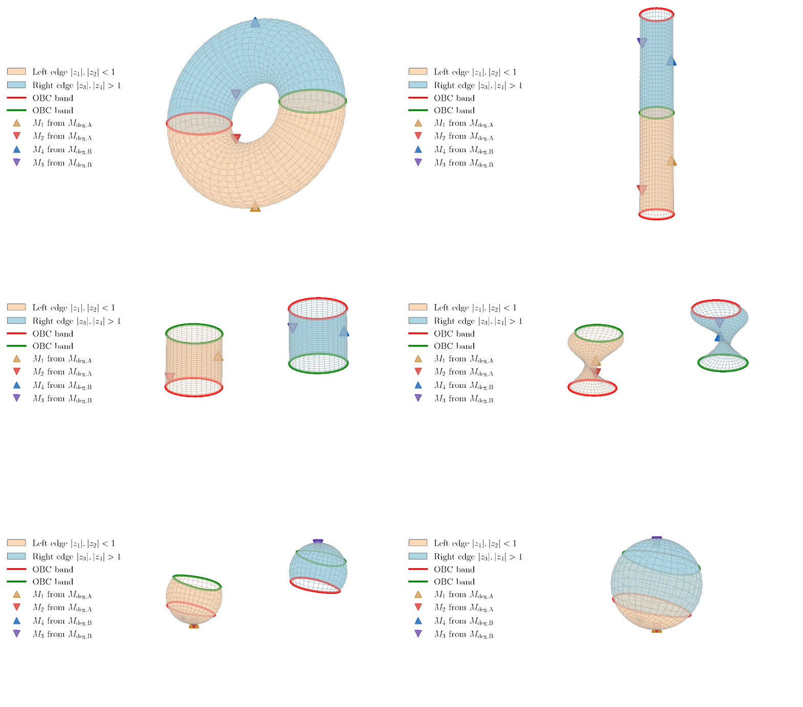
Fig 15 Band structure torus to M-Riemann sphere
Whent the cylinders from the torus is twisted into a sphere, the points where it pinches are the \(M\)-plane branch points. In this model, there are four of them. These branch points help us keep track of where the relevant \(M_i\) regions are when the torus is mapped to a sphere, which helps us check whether the bulk degeneracy point is in the correct region for edge states.
Closing thoughts
One of the takeaways from our work is that the complex band structure is important even in Hermitian systems. This complex band structure also underlies many other physical phenomena. While our proof is for nearest neighbour models, many of the analytical tools and arguments can be extended for longer range models.
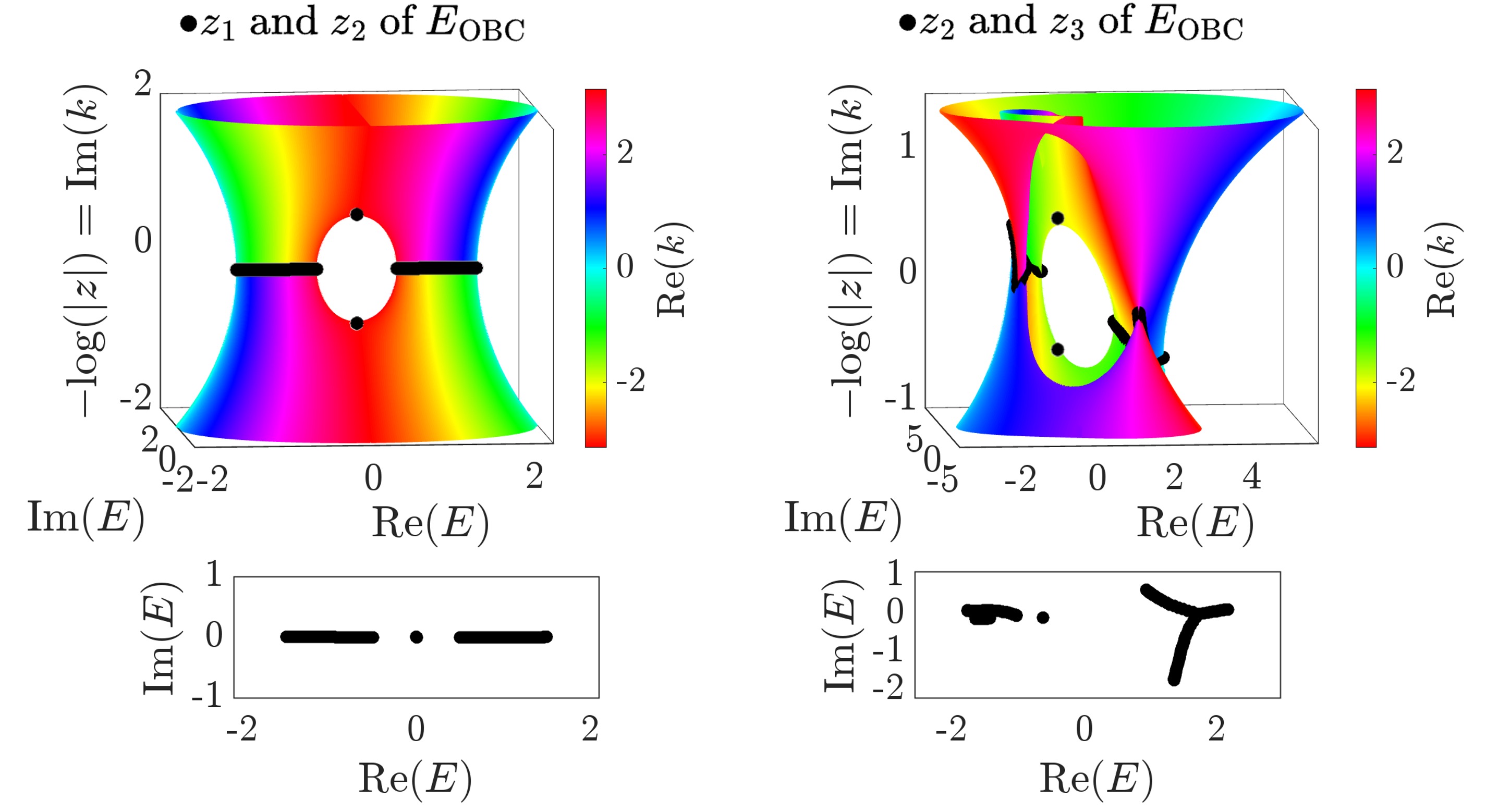
Fig 16 Complex band structure for SSH and the asymmetric non-Hermitian model in our paper.
Above is a pretty picture of a complex band structure from the Supplementary Material in our paper. It is based off the Appendix A section of Heming’s tutorial which also explains many of the other algebraic tools used in our work. Also check out Dali’s experimental measurement of the complex band structure.
I thank my co-authors Heming, Sasha and Shanhui in this work. In particular, many of the algebraic formulas and the proof for our topological invariant originated from co-first author Heming.